Building a forecast model to predict the Caspian Sea level
by Klaus Arpe
The Caspian Sea (CS) is the world’s largest enclosed basin of water with an area of 371,000 km² equivalent to the area of the British Isles or Norway, and a volume of 78,200 km³. Its main source of water is the Volga River, but it also receives water from the Ural, Kura, Terek and Sefidrud Rivers (fig. 1). Its sea level lies below the mean sea level of the oceans and has varied between -25 to -29 m over the last 150 years with a much faster responding change in water level over the last century in comparison to global sea level changes. Since the 1960s, the artificial regulation of the inflow of the main rivers feeding the Caspian Sea have intensified and as a consequence, the natural river input to the water budget of the Caspian Sea level (CSL) has changed.
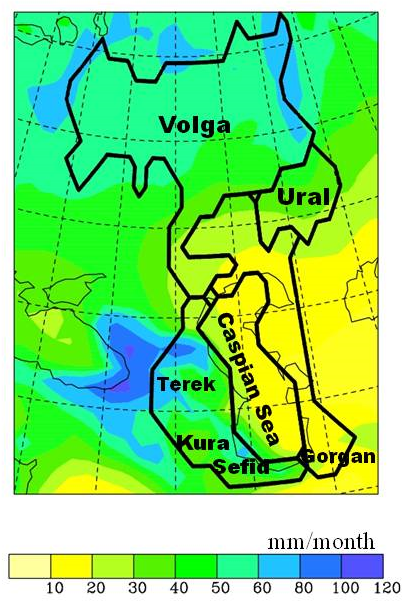
Fig. 1: Different catchment areas in heavy black lines and annual mean precipitation colours. Units in mm/month.
Because of the large socio-economic impacts of CSL changes, several attempts at forecasting them have been made, the first one in the early 1940s by Kalinin (1941).
This method based on a water balance estimation was successfully implemented at the Hydrometeorological Center of Russia (HMRC).
Modified versions of the Kalinin method have been used until now to issue operational monthly CSL forecasts with up to one year lead time. A recent study by Arpe et al. (2012) investigated the CSL change using reanalysis data from ECMWF.
The positive results from that study led to the development of a simple dynamical seasonal prediction system of the CSL using ECMWF seasonal forecasts (FCST).
The positive results from that study led to the development of a simple dynamical seasonal prediction system of the CSL using ECMWF seasonal forecasts (FCST).
Building a model for the Caspian Sea Level
The data used to build the model were observations of CSL fluctuations, historical gauge data and, from 1993 onward, altimetry observations from satellites. However, uncertainties in the measurements due to large basin differences and surges up to 3 m makes the definition of a mean CSL very difficult. Precipitation (P) and evaporation (E) over continents and seas were taken from ECMWF interim reanalysis (ERAI) and FCST. The evaporation forecasts over the CS turned out to be unrealistic due to an assumption of a fixed sea surface temperature (SST) and was therefore not used. The evaporation over the continents (CS) is most likely to be overestimated (underestimated), therefore precipitation minus evaporation (P-E) was not calculated directly but the evaporation was first reduced by 5% over the continents and increased by 20% over the CS to get the mean values into better balance. Discharge data for monthly mean Volga River discharge (VRD) as well as of the Kura and Ural rivers, and the Sefidrud and Gorganrud were collected.
A simple conceptual model for water storage
The time from precipitation events until its water reaches the CS for the Volga basin is very long due to many factors: storage in the ground, snow and ice during winter, the long travel time down the river and the many dams. The dams store the water mainly for generating electricity, but also for irrigation and water consumption. The dams let the water pass according to the demand for electricity in the country. Normally the dams are full in July after the snow melt and with the increase of precipitation during summer. After that, the VRD responds to the precipitation more directly.
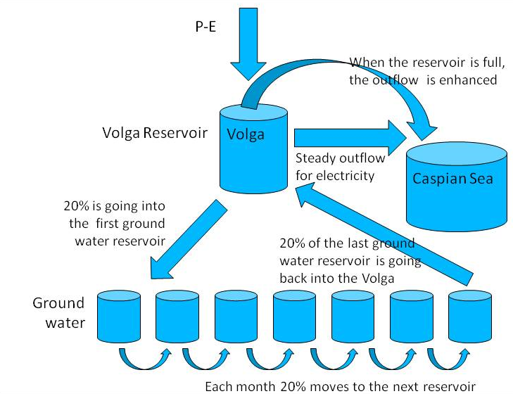
Fig. 2: Schematic of the model to parameterize the water storage in the Volga basin.
A simple model was implemented to try to simulate the storage by ice and snow in winter; it uses P-E values of up to 4 of the preceding months. This input is fed into the Volga reservoirs (Fig. 2) from which a minimum nearly constant amount of water is released due to the need for electricity. When the amount of water in the reservoirs becomes too low, this released water is reduced to avoid negative amounts in the storage. If the amount of water in the storage exceeds a maximum threshold, more water is released for discharge until the storage is back to its maximum. Moreover, a delay due to storage as groundwater is parameterized. The model was calibrated using the observed VRD data.
The effect of this delay can already be shown by comparing the Volga Basin P-E mean annual cycle with that of the observed and simulated VRD (Fig. 3). The uncorrected P-E (P-Ei) has a broad maximum from October to February while the observed VRD (VRob) has a sharp maximum in May, which is the delay due to storage in snow and ice.

Fig. 3: Annual cycle of the Volga River discharge as observed (VRob) compared with P-E over the Volga Basin from ERAI (P-E) and after other calculations. A delay due to snow and ice for ERAi (P-Ec) was applied. After that the effects of reservoirs and groundwater (VRDc) were parameterized. noGW refers to the delay without groundwater parameterization. VRD data are converted into mm/month over the catchment area.
The water budget for the CS is calculated from P-E over the whole CS catchment area with the corrections mentioned above. Direct groundwater infiltration to CS is not calculated explicitly but is being taken care of on average by investigating anomalies only.
The FCST data are treated in the same way as the ERAi data. For calculating the VRD, P-E values for up to 4 months before the current months are needed. For a forecast, the ERAi data of the months before the initial date of the FCST are used and the FCST data for the months after that. At the beginning of each forecast, the CSL data and the storage of water in the Volga Basin are taken from the simulation driven by ERAi. Observed CSL data are only used once at the beginning of the integration of the water budget, i.e. 1979. Later, only P-E values from ERAi or FCST enter the calculations. The observed VRD and CSL data are used only for validation and for tuning.
Forecasting the CSL
In Fig. 4, the CSL anomalies (mean annual cycle removed) as observed from satellite (black curve) and as simulated using only data of the hydrological budget as analysed by the ERAi up to the April 2015 (red curve) are compared. The years 2006-2015 were a period of a steady drop by 1 m, especially strong in 2010 and 2014. The estimates using ERAi data and observations by satellites deviate hardly by 10 cm in that period. Further the FCST for the next year is shown for each month since December 2014. All FCSTs predict that the CSL will stop falling in May 2015 and stay constant after that (mean annual cycle removed) all suggest the same level until beginning 2016 with a little lower value for the forecast from December 2014.We are now waiting for the next few months to see how successful our forecasts have been.
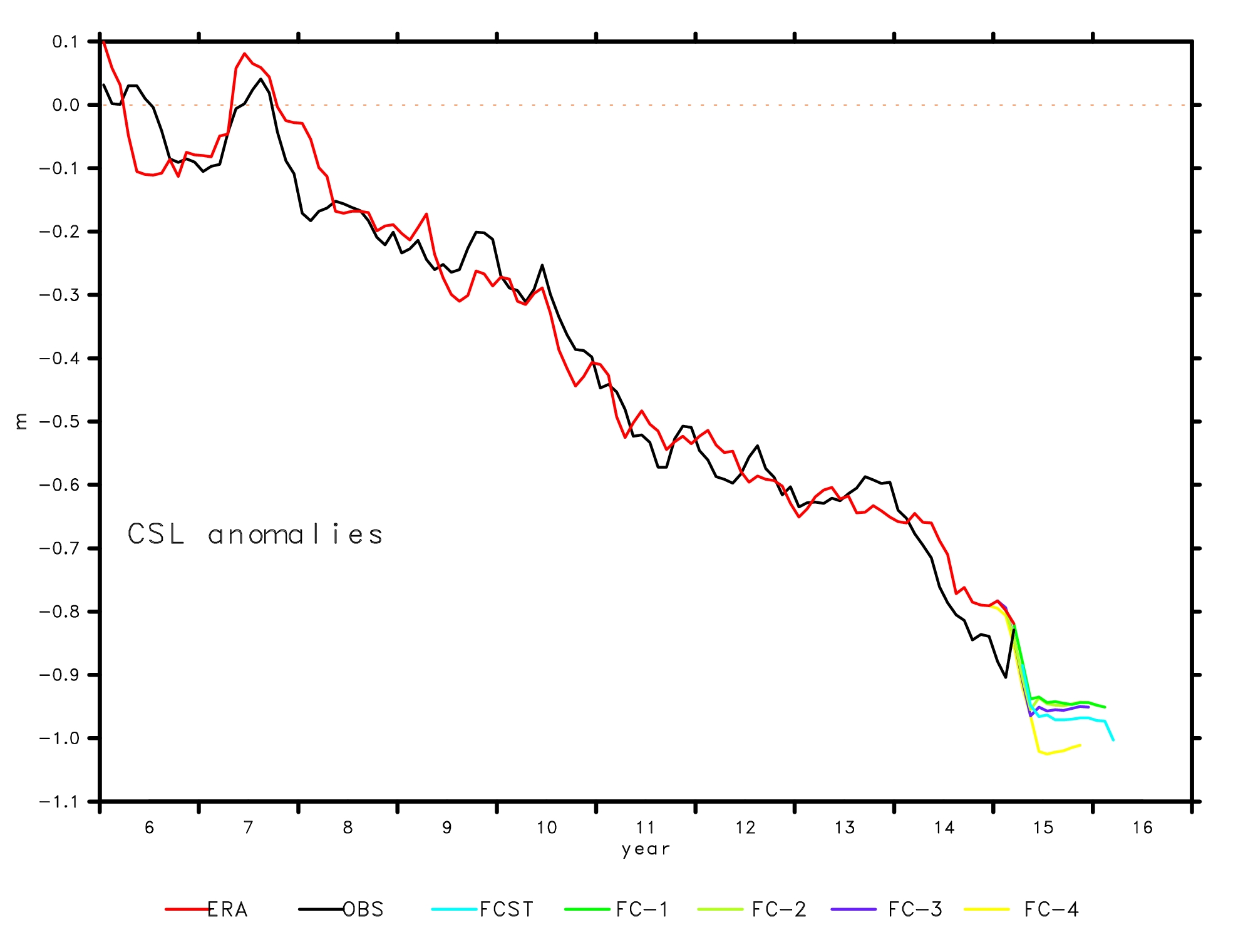
Fig. 4: Last 10 years of monthly variability of the CSL as observed from satellite (black curve) and as simulated using only data of the hydrological budget as analysed by the ERAi up to the present (red curve) without using any information of the observed CSL. All with a mean annual cycle removed. Further the forecasts for the next 12 months are shown, starting April 2015 (blue), March 2015 (green), Feb 2015 (yellow green), Jan 2015 (purple) and Dec 2014 (yellow).
This study shows that a simple conceptual model can be a powerful modelling tool for such large basins as the Caspian Sea, especially if the output is univariate. A more complex model which takes the entire basin into account would be an immense effort to develop, but would not necessarily yield a more accurate result.
References:
(2012) Impact of the European Russia drought in 2010 on the Caspian Sea level. Hydrol. Earth Syst. Sci 16: pp. 19-2
Arpe K., Leroy S. A. G., Wetterhall F., Khan V., Hagemann S. and H. Lahijani (2014): Prediction of the Caspian Sea Level using ECMWF seasonal forecasts and reanalysis. Theor Appl Climatol DOI 10.1007/s00704-013-0937-6, 201
Kalinin GP, Smirnov KI, Sheremetev (1968) Water balance calculations of the future state of the Caspian Sea level. Meteorologiya i Gidrologiya. 9: 45-52 (in Russian)
0 comments