How writing an article can come out of the blue (KGE on log-transformed flows: a bad idea?)
Contributed by Léonard Santos (Irstea, France).
It is common to read articles in which the Kling and Gupta Efficiency (KGE, Gupta et al., 2009) or its modified version (KGE’, Kling et al., 2012) are used as a metric to evaluate the quality of streamflow simulations. They are often seen as a solution to substitute the Nash and Sutcliffe Efficiency (NSE, Nash and Sutcliffe, 1970).
However, are these two criterion totally comparable? Can the KGE be used exactly in the same way as the NSE is?
I am currently ending my PhD at Irstea (France) and during this PhD I was faced with the questions above. Let me tell you the story of how the work on a big amount of data can lead to better understanding some hidden scientific questions.
This story began one year ago. I was working on model development and I tried to evaluate my work on a wide set of catchments (i.e., 650 gauged stations over France). In order to analyse the model performances on low-flows, I decided to calculate the KGE’ on the log-transformed flows. This choice seemed logical as the same transformation is used to analyse low-flows with the NSE. It was also used with the KGE by some authors. I thus trusted the ability of this metric to represent the quality of low-flows simulations.
Some doubts came when I noticed some highly negative KGE’ values on log-transformed flows in some catchments. I knew that a good performance can be inferred when the KGE’ value is over 0.8. But what is the difference between a value of -0.1 and a value of -165? In addition, how a value of -165 is even possible?
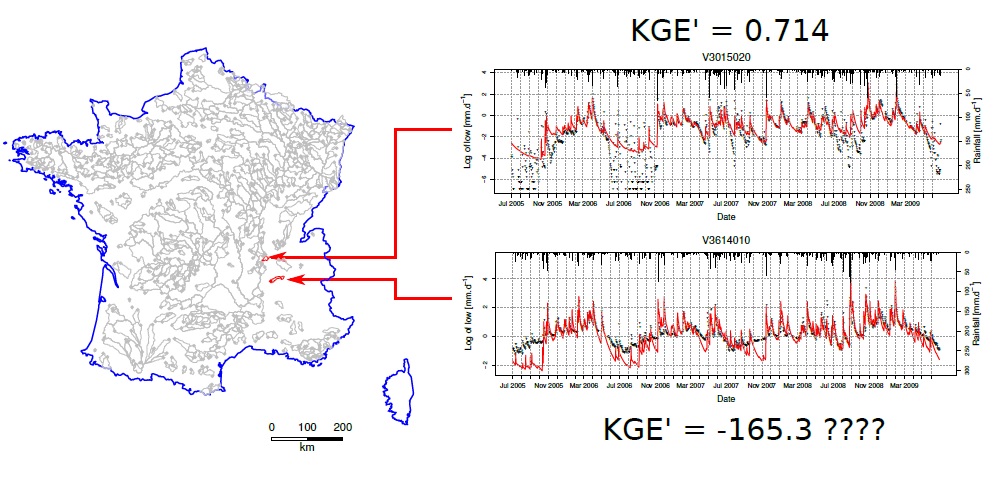
How a value of KGE = -165 is even possible? See paper: Santos et al. (2018)
Starting from this observation, I tried to analyse the mathematical formulation of the KGE’ in order to understand these highly negative values. I then noticed that the KGE’ value is unstable when the mean log-transformed streamflow (observed or simulated) is close to zero. This is more likely when the logarithm of flow is used than when no transformation is applied (because the logarithm of 1 is equal to 0 and an average flow of 1 is more likely than an average flow of 0).
The next step was then to speak about this issue with my colleagues, the members of the Catchment hydrology research group at Irstea in Antony: “Hey, has anybody ever faced this issue?”
And the answer was… they had not!
However, the discussion allowed to understand that the issue was even worse. The discussion with my colleagues can be summarized by the following quotes from different members of the team:
- Alban De Lavenne (in his office): “Yes, it is a problem, but I wonder why we do not use the nth root of the flow, it allows to avoid issues with zero flows.”
- Maria-Helena Ramos (in the metro): “If you use litres per second instead of cubic meters per second, it will solve the issue! :-)”
- Laure Lebecherel (before the metro, in the bus): “Wait a minute… The metric value is not expected to change when the flow dimension is modified???”
As a result of these fruitful discussions, I noticed that, in addition of being unstable, the KGE and the KGE’ criteria are not dimensionless when the logarithm transformation is used.
After that, given that the logarithm transformation is used in some papers, my “senpai” (Dr. Guillaume Thirel) decided that we needed to publish on the findings to warn the hydrological modellers’ community. We chose to make a technical note, which seemed well adapted to this type of manuscript.
We submitted a manuscript to HESS journal. It was quite well received by both editor (Bettina Schaefli) and reviewers (Lieke Melsen and Björn Guse) and the open discussion even provided an interesting solution to replace the logarithm (see, mainly, the comments by John Ding).
The story had a happy ending with the publication of the technical note in the journal last 30 August. All the details and the interesting discussion can be found here.
However, the lesson to be learnt here is not only that the use of the logarithm transformation to calculate the KGE needs to be used carefully.
The main purpose of this blog post is to underline that this study and the results obtained were possible because I was using a great amount of data (i.e., a large data set of catchments). It thus remind us of the usefulness of using large dataset in hydrology.
Also, it shows that a paper is not necessarily the result of a long-term publication plan. It can also come from a side issue arising during the research work and, most importantly, after openly discussing with colleagues and exchanging ideas.
References:
-
Gupta, H. V., Kling, H., Yilmaz, K. K., and Martinez, G. F.: Decomposition of the mean squared error and NSE performance criteria: Implications for improving hydrological modelling, J. Hydrol., 377, 80–91, 2009.
-
Kling, H., Fuchs, M., and Paulin, M.: Runoff conditions in the upper Danube basin under ensemble of climate change scenarios, J. Hydrol., 424–425, 264–277, 2012.
- Santos, L., G. Thirel, and C. Perrin: Technical note: Pitfalls in using log-transformed flows within the KGE criterion. Hydrol. Earth Syst. Sci., 22, 4583–4591, 2018.
November 7, 2018 at 19:10
Léonard (and Irstea team), thanks for the smooth story, important scientific outcome, and for highlighting also the added-value from large sample hydrology. To me, these numerical artefacts of KGE on log-transformed flows limit the potential for comparison of model performance at different catchments (particularly including catchments with the flow characteristics you stated) which was one of the drivers for proposing the KGE metric. Overall, thumps up for this investigation!
November 8, 2018 at 00:50
Nice blog and nice paper! I commend the authors and others at Irstea for always making the distinction between using KGE (as originally proposed in Gupta et al., 2009) and the modified version by Kling et al., (2012), KGE’ or KGE2 or KGEmod, as you sometimes find it written. In case of interest to others, I went back again recently to the Kling et al paper to find the motivation for modifying the variance ratio to using coefficient of variation. They state this modification “ensures that the bias and variability ratios are not cross-correlated, which otherwise may occur when e.g. the precipitation inputs are biased”. Additionally, I’ve noticed in several papers that authors don’t state which version of the KGE they use; or write the equation for the modified version but only cite the original paper, and vice versa. It is my opinion that we should be explicit when using it. A minor point but as we see from the finding presented on log transformation with KGE from Léonard and coauthors, small differences can be important in unexpected circumstances. Plus it’s good practice for making our science more reproducible! Cheers, Shaun.
November 12, 2018 at 02:44
Nice post – definitely thought provoking. I think of the log transform for flow as being aggressive, and colleagues who use transforms in developing statistical prediction models on zero-bounded variables often use square & cube roots for normalization instead. In any case, I think it sets a nice example that you diagnosed your score outcomes. In the days of easy verification packages (R, python, etc.), that’s not always the case. We’ve started using KGE more after re-reading Hoshin’s 2009 paper (thanks to Martyn C, tbh), but I do worry about the effectiveness of scores that are unbounded on one end of their range (ie KGE, NSE) in optimization applications (eg parameter estimation), especially across a collection of sites where some may be in the negative zone (with strong KGE performance gradients) while others are positive (with weak gradients). Perhaps a topic for a different blog!
November 12, 2018 at 10:04
Ilias, thanks for the discussion on the article this last Nov 1st. It helped me finding an interesting way to tell this story.
November 21, 2018 at 15:04
Dear Shaun, thank you very much for the comment. I agree with you that it is important to mention the used version of the KGE. Indeed, there may be differences between the two versions of the score and I am curious to see an analysis about these differences in hydrological modelling application (as far as I know it does not exist in the literature).
Dear Andy, thank you for sharing your thoughts. I understand that the use of transformations such as the logarithm or the inverse of flows can be aggressive and constrain a lot the models. However, in my experience, it seems that models that are calibrated using the log or the inverted flows in the objective function are better to reproduce the lowest part of the flow duration curve than models calibrated using the square root (maybe for the wrong reason, I don’t know…). Regarding the unbounded aspect of the KGE and KGE’, I agree that it can represent an issue for parameter calibration. I can add, that one of my colleagues observed that it is also an issue when applying classical sensitivity analysis techniques (i.e. Sobol or Morris).
November 28, 2018 at 14:02
Dear Leonard, I enjoyed reading this post.
Recently I encountered an issue with the KGE when I tried to assess the quality of modelling lake levels. I had already seen in some graphs that the model showed a substantial bias. However, the Beta (bias) component of the KGE still came up as 1.01, 0.99, for even the worst periods. It took me some time to realize that this is because lake levels are on an interval scale (no true zero); The ratio between modelled mean levels of 419 or 418 m.A.S.L. is close to one, but the bias of 1m is large if the dynamic range is only ~5m or so.
Reflecting on the physical meaning of the bias term as an estimation of the water balance, I now like how beta is implemented in the python package spotpy as sum(simulation)/sum(observation) instead of means. Comparing the means of two series of water levels makes sense, but comparing the sum of those series does not.
Clearly, I would have been less surprised if I had read your technical note directly after this post came out 😉