If you had to build a probabilistic streamflow forecasting chain from scratch, what components would you pick up?

Contributed by Joseph Bellier

Take a meteorological ensemble, use it as input of a hydrological model, but then what? There are many ways to improve a forecasting chain, but which upgrade is going to be the most beneficial? We recently published a paper in which we “play” with a modular forecasting chain, by adding/removing various components and verifying how skillful the streamflow forecasts are. Here are some outputs.

The ensemble approach, in its wider definition (not only meteorological ensemble forecasting), is an elegant way to generate probabilistic forecasts. It “samples” within what’s uncertain (initial conditions, model parameters and structure, etc.), to then generate simulations based on equations that simulate physical processes. It results in probabilistic predictions whose uncertainty is “dynamic”, in the sense that it is specific to each forecast case. And that’s what decision makers like. 

But generating ensemble streamflow predictions that are reliable requires to combine various ensemble techniques that tackle all the main sources of uncertainty. For instance, I remember the study of Thiboult et al. (2016), who combined meteorological ensembles, hydrological data assimilation (to provide an ensemble of initial model states) and a hydrological multi-model, to generate streamflow forecasts with 50,000 members. While this is highly interesting from a science perspective, it still seems unaffordable for most operational forecasting centers.

This is where statistical corrections come into play. For us hydrologists, we usually refer to pre-processing and post-processing the correction of the meteorological forecasts and of the streamflow forecasts, respectively. I like to see the pre-processing as an “amplifier” of the meteorological signal, to make sure it is strong enough to pass through the hydrological model, and the post-processing as a “last chance” correction that ensures the reliability of the output streamflow forecasts (treating the hydrological uncertainty mostly, but also any other source of uncertainty that remains).

A pragmatic approach to obtain good streamflow forecasts is therefore to combine ensemble-based techniques with statistical corrections. But each of these components has a cost, which can be financial (access to meteorological forecasts), scientific (skills required to develop the algorithms and ensure their support), or computational (resources for running ensemble simulations), so being able to prioritize their development is highly valuable.

In a paper that we (G. Bontron, I. Zin, and myself) recently published, entitled Selecting components in a probabilistic hydrological forecasting chain: the benefits of an integrated evaluation, we start from a “baseline” forecasting chain, which simply comprises a meteorological ensemble (the ECMWF) and a hydrological model (GRP), and we gradually introduce more sophisticated components, either based on the ensemble approach (meteorological grand ensemble, hydrological multi-model) or on statistical corrections (pre-processing, post-processing).

We evaluated the streamflow forecasts obtained with the 3 x 2 x 2 x 2 = 24 possible combinations of components, on 6 basins located on the French upper Rhone River, and using a variety of metrics.

First of all, it has been comforting to see that at each stage of the chain it was always the most sophisticated component that gave the best results on streamflow, no matter how complex the rest of the chain was. In other words, it means that modelers can work on their own to improve a specific component (e.g., a pre-processing), and it will most likely be beneficial on the final streamflow forecasts.

But then, we wanted to study some specific questions that are of interest for someone who wants to build a forecasting chain from scratch.

For instance, there is strong debate in the hydrological forecasting community about the need of two statistical corrections. In 2015, M-A Boucher wrote a blog post whose title was “Pre-, post-processing, or both?”. She mentioned several papers (Kang et al. 2010; Verkade et al., 2013; Zalachori et al., 2012) that had investigated the issue, and they were all concluding that the benefit of pre-processing vanishes almost entirely after post-processing is applied.

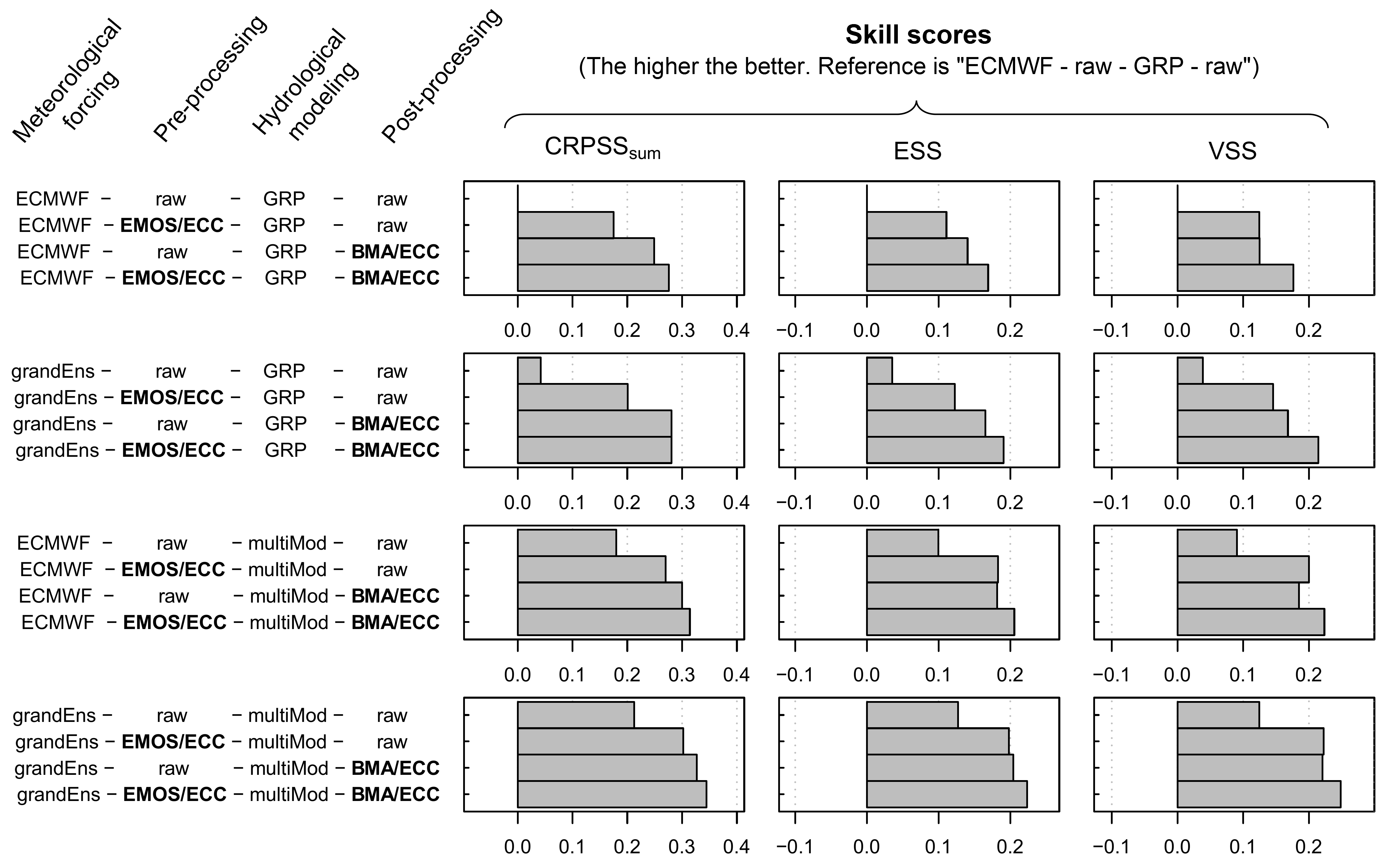
In our case study, we have found that if only one correction should be implemented, that’s indeed the post-processing. And since it is the only component able to guarantee the reliability of the final streamflow forecasts, its implementation should be systematic. However, unlike the above-mentioned studies we have found the pre-processing to remain systematically beneficial, even when combined with sophisticated components at the other stages of the chain.

Of course, this finding is probably case study-dependent. Some catchments have a more pronounced non-linear behavior than others, and the quality of the raw forcing vs the method used for statistical correction can play in favor of the pre-processing, or not.

One noticeable comment though is that at least two of the three studies mentioned above used the Schaake shuffle technique for reconstructing the multivariate dependence structure that is being lost through the statistical correction. But several papers showed that the standard Schaake shuffle suffers from several drawbacks when applied to precipitation, to the point that the benefit of the whole pre-processing may disappear. In our study we used the ensemble copula coupling (ECC) technique instead, and this is perhaps a reason why our pre-processing remains beneficial.

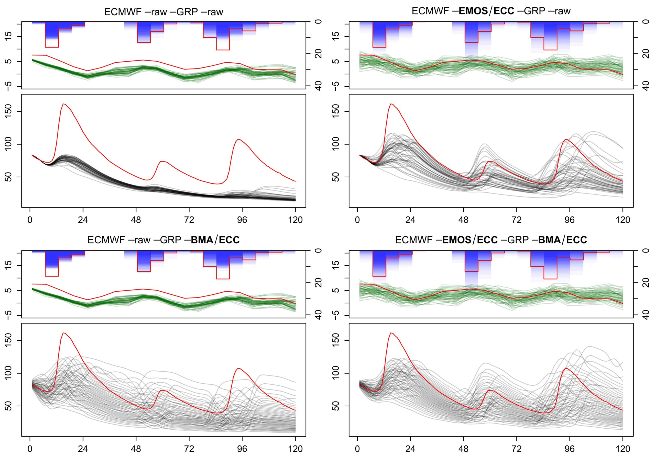
Finally, looking at individual forecasts is always insightful to better understand the role played by the different components of a chain. In the example below, the streamflow forecast without any correction (upper left) remains almost flat the whole time, despite three noticeable rain events. Pre-processing alone (upper right) amplifies the meteorological signal enough so that the hydrological model reacts, while post-processing alone (lower left) takes a different approach, increasing the dispersion of the forecast to a great extent (to correct for an under-dispersion), but smoothing out the dynamic of the event. Finally, coupling both the pre- and the post-processing (lower right) allows to increase the dispersion, while leaving the dynamic of the event obvious for the forecaster.

In our paper we also investigate other problematics, such as:

• Does the gap in skill between different meteorological ensemble forecasts (e.g., ECMWF, GEFS) persist as the rest of the forecasting chain complexifies?
• What is the best strategy, to account for the meteorological uncertainty, between a grand ensemble and a pre-processing (or both)?
• What is the best strategy, to account for the hydrological uncertainty, between a multi-model and a post-processing (or both)?

For more info:

Bellier, J., Bontron, G., & Zin, I. (2021). Selecting components in a probabilistic hydrological forecasting chain: the benefits of an integrated evaluation. LHB, 107(1). DOI: 10.1080/27678490.2021.1936825