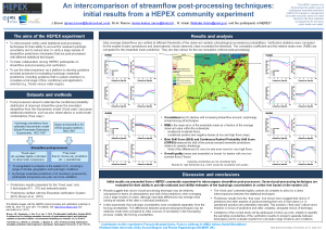
Intercomparison of streamflow post-processors Post-Processing hydrologic model simulations (Phase 1)
Contributed by James Brown, Nathalie Voisin and Maria-Helena Ramos
The experiment was launched in June 2012 and the first results are currently being anlaysed.
See our poster presented at EGU 2013:
Posters HS4.3/AS4.20/NH1.13 – Ensemble hydro-meteorological forecasting for improved risk management: across scales and applications
Our aims is:
- To establish the advantages and disadvantages of different post-processing techniques and strategies when accounting for hydrologic uncertainty
- To foster ongoing collaboration among the HEPEX participants on the topic of streamflow post-processing and verification
- To use the intercomparison work as a platform to develop more broadly applicable frameworks for evaluating hydrologic ensemble predictions, including frameworks that are system-oriented (i.e. consider a full range of flow conditions) and application-oriented (e.g. for floods versus water supply)
This initiative began with the HEPEX post-processing and verification workshop in Delft, NL, from 7-9 June 2011, for which a science plan was drafted. Two teams were organized during the workshop (a post-processing techniques team and a verification techniques team) and several proposals were made for follow-up work. This experiment identifies a limited number of scenarios for inter-comparing streamflow post-processors and launches an open call for participation among those who attended the recent HEPEX workshop to run those scenarios. A second phase of the intercomparison will focus on post-processing hydrologic ensemble forecasts that comprise a combination of hydrologic and forcing uncertainties.
Data are provided for 12 unregulated river basins in the eastern part of the United States. Streamflow observations and hydrologic model simulations come from the Model Parameter Estimation Experiment (MOPEX). Daily discharge simulations were generated by 7 different hydrologic models. Simulations were performed with calibrated model parameters. The simulation period covers 36 years, from 1962 until 1997. The experiment comprises several scenarios for participants to consider, including scenarios with fixed options for straightforward intercomparison and free choice to accommodate participants’ experience and ingenuity.
For additional information, contact us:
James Brown
Nathalie Voisin
Maria-Helena Ramos

April 11, 2013 at 10:30
I like the initial results of the study in particular how similar they are. The evaluation you show does not include a measure which is focused on individual percentiles e.g.how do the correction methods impact the 90th percentile? Please also note that ECMWF has no problem in being identified.
April 18, 2013 at 17:56
Hi Florian,
Each plot shows the verification scores for a wide range of streamflow thresholds that are defined by their climatological exceedence probabilities. Thus, looking at the domain axis on each plot, a value of 0.1 corresponds to a daily observed streamflow threshold that is exceeded, on average, once every 10 days. The precise interpretation depends on the metric considered. For example, the BSS is measured with respect to the exceedence of the discrete threshold identified (it is a dichotomous measure). The CRPSS is measured over the subset of pairs (predictions and observations) for which the observed value exceeds the threshold.
Other interpretations of the “90th percentile” are possible, such as the reliability of predictions issued for a discrete event (e.g. flooding) with a probability of ~0.9.
In due course (for any papers), verification results will need to be produced conditionally on a range of attributes, including observed and predicted amounts, seasons etc. Feedback on specific verification strategies or approaches to ensure a broad and fair intercomparison would be welcome from the project participants or others.
Cheers,
James
January 17, 2014 at 19:26
I think it’s interesting that the performance was so similar for the various approaches, and I wonder if that has partly to due with the the raw simulations being fairly well calibrated (I’m speculating). Does the spread in performance depend on the quality of the raw model performance? In any case, nice work, and I’m looking forward to phase II. -Andy
January 19, 2014 at 23:51
Hi Andy,
Thanks for the reminder! We do have contributions from various folks to do a good analysis, I think. We just need to find the time to finalize the verification/analysis (accounting for the sampling uncertainties too) and write it up.
Yes, I think the models are fairly well-calibrated in most basins. On the one hand, this may lead to stronger similarities between techniques. On the other hand, a smaller fraction of the overall skill should come from the climatological portion of the bias correction, which is going to be an issue with a poorly calibrated model, and any post-processing technique should do this well. Other controls include the choice of predictors and basin characteristics. For example, in basins with very strong memory, the use of the prior observation is likely to be more important than the details of how the joint distribution is modeled. There’s a decent range of basin characteristics and variability in forecast quality across the basins considered, I think. Indeed, in some basins, the differences between techniques are greater than in other basins.
Also, the first scenario imposed rather tight controls on how the post-processors were formulated, in an attempt to isolate the contribution of modeling technique, rather than all sources of variability in real-world applications. Not surprisingly, completely free choice in the way the post-processor is formulated (the second scenario) also leads to important differences. Thus, in a less controlled environment (read: operational forecasting), there are opportunities for an experienced forecaster to gain additional skill through careful application (i.e. choice of predictors, data stratifications etc.) or to lose skill through poor application. Also, this study will not consider all aspects relevant to operational forecasting, such as the ability to preserve temporal statistical dependencies in the ensemble traces or practicality/data requirements; it’s a start though.
James