Recent development of post-processing methods in short-term hydrometeorological ensemble forecasting

Contributed by Wentao Li and Qingyun Duan 

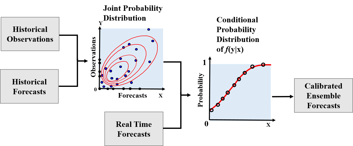
Due to various uncertainties in model inputs and outputs, initial and boundary conditions, model structures and parameters, raw forecasts from meteorological or hydrological models suffer from systematic bias and under/overdispersion errors and they need to be corrected before being used in applications. Various statistical post-processing methods have been developed to correct these errors and achieve “sharp” forecasts subject to “reliability”. As in the book “Statistical methods in the atmospheric sciences” by Wilks, statistical post-processing methods can be generally divided to two categories from the view of statistics, namely regression-based methods (e.g., ensemble MOS and logistic regression) and kernel density-based methods (e.g., BMA and ensemble dressing). An example of the flow of a regression-based statistical post-processing method is shown in Figure 1. As there is already a review of post-processing in a previous blog in 2013,  in this blog post we discuss several newly developed post-processing methods for short- to medium-term hydrometeorological forecasting.

As described in several papers (e.g., Scheuerer et al., 2015), there are several difficulties in post-processing variables such as precipitation and streamflow/river stage: (1) these variables follow a mixed distribution of a positive probability at zero value and a skewed continuous distribution for non-zero amounts; (2) the heteroscedasticity problem, namely that the forecast uncertainty increases with the magnitude of forecast variables; and (3) the representation of spatio-temporal and inter-variable dependency, which is important for applications such as hydrological forecasting.

To model the hydrometeorological variables with skewed distribution and non-homogeneous variance, one common treatment is to apply transformations to normalize the variables and stabilize the variance. After the transformation, traditional statistical models under assumptions of Normal distribution and homogeneity can be applied. Examples of the transformations include the Box-Cox or power transformation in heteroscedastic censored logistic regression (HCLR) and the log-sinh transformation in Bayesian joint probability (BJP). Moreover, there are also post-processing models that directly use non-Gaussian distributions without any transformations, such as the censored, shifted Gamma (CSG) distribution-based EMOS by Scheuerer and Hamill (2015). To deal with the heteroscedasticity problem, EMOS model includes the ensemble spread of raw forecasts as predictor to adjust the non-homogenous forecast uncertainty. R packages such as “ensembleMOS” and “crch” have made it easy to apply these methods.

How to model spatio-temporal and inter-variable dependency of hydrometeorological variables has gained much attention in recent years. To solve this problem, several “shuffling techniques” have been developed, namely to “shuffle” the ensemble members generated from the post-processed probability distributions according to some “rank structures” which represent the spatio-temporal and inter-variable dependency. Among these methods, the Schaake shuffle are mostly applied, in which the ensemble members are reordered according to the “rank structures” obtained from historical observation archives. However, the drawback of Schaake shuffle is that the templates from past observations may not represent the current synoptic situation.

Recently, two types of Schaake shuffle variants have been developed. One type is the ensemble copula coupling (ECC) scheme developed by Schefzic et al. (2013). ECC reorders ensemble members according to the “rank structures” of raw ensemble forecasts, thus accounts for the multivariate rank structure information of the current synoptic situation. The other type of variants select the “rank structures” from a subset of historical observations under “similar” situations using synoptic analogs or other similarity criterions. This type of method includes the “SimSchaake” by Schefzic et al. (2016), the minimum divergence Schaake shuffle (MDSS) by Scheuerer et al. (2017) and the meteorological analogues-based Schaake shuffle by Bellier et al. (2017). Wu et al. conducted a comparison experiment of the three schemes of shuffling techniques, namely the original Schaake shuffle and its two types of variants.

Besides this progress, what challenges remain for post-processing? A 2013 blog post by Nathalie Voisin, Jan Verkade and Maria-Helena Ramos (here) included a list of challenges for post-processing, many of which still need to be worked on. We also recommend this chapter by Dr. Thomas M. Hamill, which also emphasizes several challenges in post-processing, such as developing post-processors suitable for limited training data, and sharing post-processing software and data together “to build a postprocessing community”.

What other challenges do you think exist in post-processing? We welcome your comments on your experiences and opinions of post-processing below.

You can find the full review on statistical postprocessing methods for hydrometeorological ensemble forecasting in the authors’ recently published review paper:

Li W, Duan Q, Miao C, et al (2017). A review on statistical postprocessing methods for hydrometeorological ensemble forecasting. WIREs Water, e1246.