The importance of parameterizations for better continental forecast systems
Contributed by Luis Samaniego (Helmholtz Centre for Environmental Research – UFZ)
Parameterization: An old, ubiquitous, and recurring problem
Modeling is a complex human activity because of the crucial trade-offs that have to be made to reach a final objective. According to Popper [1935], modeling is an interactive research process that starts with the observation of a natural system (e.g., the water cycle) aiming for a “mental” abstraction of the main elements that are necessary to faithfully describe the evolution of the system over time. Abstraction implies a reduction of the system complexity, which is often formalized as a set of equations, which we call a model. Consequently, a model constitutes an elaborate hypothesis of the dynamics of the system that should be falsifiable. In other words, predictions should be confronted with new data to establish the ability of the model (skill) to reproduce them.
The various kinds of numerical weather prediction models (NWP), land surface schemes, and hydrologic models (HM) that exist today are the result of a continuous and elaborate formalization process that has led to a set of equations based on fundamental physical principles whose numerical solution is possible nowadays by means of sophisticated algorithms. This modus operandi has not changed much since 1922, when L. Richardson wrote his seminal book in which the foundations for numerical weather forecasting were set down. A similar approach was employed by Freeze and Harlan [1969] four decades later for the formulation of the blueprint for a “distributed” hydrologic model.
What changed dramatically since 1945 is the speed at which numerical algorithms can be solved. Since the advent of the first electronic computers (e.g., the ENIAC), the skill of general circulation Models, numerical weather prediction models (NWP), land surface models (LSM), and hydrologic models (HM) has been mainly increased by improving their dynamical formulations (conceptualization), the numerical analysis, and/or by doubling resolution as the storage capacity and computational power allowed (e.g., Global Climate Models employed in IPCC Assessment Reports have doubled every five years since 1990) [Lynch, 2008]. It should be noted that an increase of the model resolution by a factor of two implies about ten times as much computing power. Recent visions that have emerged in hydrologic modeling (e.g., hyper-resolution initiative) seems to follow this pathway [Wood et al., 2011, Bierkens et al., 2014].
Despite the above improvements in model development, it should be noted that “there are always scales and physical processes that can not be represented by a numerical model, regardless of the resolution”. Parameterization is the “process by which these important processes that can not resolved directly by a numerical model are represented” [Stensrud, 2007]. Put differently, parameterization is a simplified and idealized representation of the physical phenomenon at a given scale. These simplifications usually require new variables and numerical constants, often called parameters.
Model parameterizations, on the contrary to model development, have changed little during the past decades. In 1922 Richardson already recognized that the theory and “constants” (what I denote as global parameters below) “must be appropriate to the size” of the grid element Richardson [1922, p. 9]. He also suggested that these constants should be found experimentally (e.g., p.108), if possible. Nowadays, many of these constants are still confined in model equations as noticed by Mendoza et al. [2015] in the NOAH-MP model. Writing models and source codes with hard coded parameters is an old practice [see e.g., Crawford and Linsley, 1966] with very negative effects on results because they hinder the possibility to explore their sensitivity on model outputs and the possibility to infer them using observations.
Multiscale parameterization
Quite recently, Shuttleworth [2012, p.374] suggested that the basic parameterization of hydrologic processes in LSM (e.g., infiltration, surface runoff, snow) should be improved by representing the effects of the subgrid variability of soil properties, topography, and vegetation using statistical approaches. Gupta et al. [2014] postulated that hydrologic modeling should pursue “generality” and that the hydrologic community should shift the focus away from site-specific parameter estimation towards the development of regionalization methods. As Gupta et al. put it: the benefit of a regionalization method stems from the fact that it “regularizes the optimization problem, providing constraints that greatly reduce the degrees of freedom (number of unknowns to be inferred) to a relatively small number of regional transfer function coefficients”.
These ideas were precisely the objective that motivated the development of a parameterization concept that should allow us to reduce the predictive uncertainty and enable to make hydrologic predictions across locations and scales, without the need of computational-demanding “recalibration”. The result of this enterprise was called “Multiscale parameter regionalization” (MPR) [Samaniego et al., 2010b]. In addition of regularizing the optimization problem, the MPR technique takes into account the subgrid variability of the essential aspects of the physical process that represent a given model parameter (e.g., soil porosity). By doing both steps within the model, the predictions in ungauged locations also improved.
Testing MPR
Based on current hydrologic parameterizations, we had to develop an entirely new kind of model to test the MPR hypothesis. A key aspect during the development was how to incorporate existing information gathered at different scales without ad hoc simplifications. The final product was called the mesoscale hydrologic model, mHM (www.ufz.de/mhm ). Following Klemeˇs [1986a], we devised three cross-validation tests: a) across locations, b) across spatial scales, and c) across temporal scales.
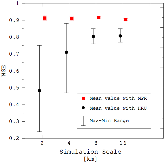
In addition to that, we provided evidence in a number of publications that quasi-scale invariant global parameters in the context of MPR lead to flux-matching across scales. So far, these tests have been carried out in hundreds of river basins in Germany, USA, and Pan-EU [Samaniego et al., 2010a, 2012, Kumar et al., 2013b,a, Samaniego et al., 2014]. As an example, Figure 1 clearly shows that an alternative parameterization method such as the Hydrologic Response Units (HRU) is not scale invariant, meaning that their parameters are not transferable to resolutions (or scales) other than those used during their calibration. The model based on such parameterization technique requires re-calibration at every scale of application, separately, leading to a huge computational load.

Figure 1: Median and interquantile range of the NSE depicting the discrepancy of 200 simulations between streamflow estimated with parameters obtained at a given scale and those obtained with parameters from other resolutions in the Neckar basin in Germany. Free parameters estimated at given simulation scale (shown in the abscissa) were used as baseline for the selected scale. Two parameterization methods are compared: MPR and HRU. Based on Kumar et al. [2013b].
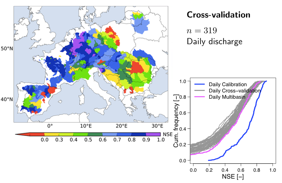
Using MPR, it has been possible to estimate global parameters simultaneously in ten randomly selected river basins that are able to reproduce streamflow in over 319 Pan-European without recalibration at a spatial resolution of 0.25◦ × 0.25◦ (see pink line in Figure 2). The basins’ area vary from 100 km2 to 50 000 km2. As a reference, the blue line indicates the CDF of the NSE obtained after calibration at every basin separately. The performance in a given location is better than the compromise solution (shown in pink), but the later, in turn, is by far a better estimate than those obtained at a single location that is transferred everywhere else (cross-validation test results shown in grey lines).
This figure also depicts that the performance of mHM in the cross-validation tests indicate that 50% of the basins exhibit a median NSE efficiency greater that 0.5. Low NSE values are related to basins having a very low raingage density and/or having strong anthropogenic influence.

Figure 2: Performance of a compromised solution over 319 Pan-EU basins. CDF depicting performance of the compromised solution (pink), the cross-validated single site performance (grey), and at-site calibration results (blue). Based on Samaniego et al. [2014].
The parameters used for the compromised solution depicted in pink also allows to reproduce the total water storage anomalies observed by GRACE at a spatial resolution of 1◦×1◦ very well. Another advantage of this method is that it allows to make simulations without discontinuities in distributed variables such as soil moisture and actual evapotranspiration. This is a typical problem occurring when a model is calibrated basin-wise. All these improvements in model parameterization will contribute to increase the forecasting skill of the model. But this is not the end of this story: better parameterizations of a LSM will improve the predictions of the NWP models due to the number of complex non-linear feedback mechanisms.
Currently we are expanding our efforts in implementing the MPR technique into the land-surface model NOAH-MP to demonstrate the applicability of this technique in the context of this LSM [Thober et al., 2014], which is part of the WRF-HYDRO system. Eventually, we expect that parameterizations based on the MPR technique would contribute to reduce the predictive uncertainty of WRF-HYDRO and similar systems.
Acknowledgements
I thank the constructive comments provided by Rohini Kumar, Stephan Thober, and Olrich Rakovec.
0 comments