Get your geek on: handling data for ensemble forecasting
Contributed by James Bennett, David Robertson, Andrew Schepen, Jean-Michel Perraud and Robert Bridgart, members of the CSIRO Columnist Team
There’s something about discussions of data handling that’s particularly soporific – but don’t nod off yet!
Most hydrologists are trained to work on individual catchments and we often opt for simple conceptual models. In the pre-ensemble era, we were often quite happy to use unsophisticated ways of crunching numbers: many of us can remember (perhaps quite recently!) using desktop computers to tune and run models, storing data in text files, and so on.
Maybe it’s because it’s obvious, but it’s little remarked that switching from deterministic forecasts to ensembles means handling much more data. Here at CSIRO we tend to use 1000-member ensembles, and our partners at the Bureau of Meteorology use a method that generates 6000 (!) ensemble members for each forecast. If you’re running cross-validation experiments across multiple catchments this can lead to migraine-like data headaches.
In a recent experiment for 22 catchments we generated over 2TB of rainfall and streamflow hindcasts. Of course generating the hindcasts is only one step in the process –verifying them with a bunch of different tests and generating a load of plots can be even more time consuming. It’s simply not feasible to run experiments like this without getting your geek on [1], putting on your “big data” cap (backwards of course) and taking advantage of the awesome power of computer science.
Computer power and data storage
We first began developing a national seasonal forecasting service about 8 years ago. While seasonal forecasting is far less computationally intensive than, say, daily forecasting, we still hit the limits of what could be achieved with desktop computers. So we farmed out jobs to HTCondor, a system that scavenges unused processing power from the many desktop computers at CSIRO. More recently, we have been writing software for applications in short-medium term forecasting that takes advantage of parallelisation in CSIRO’s high-performance supercomputers.
Data storage is another crucial issue. A few years ago we got sick of storing and exchanging thousands of voluminous text files of differing formats and unknown provenance and repute, and followed the climate community on the path to data righteousness: netCDF.
netCDF is a self-describing binary file format that is purpose designed for multi-dimensional data. It’s traditionally been used by ocean and climate modellers, and has a very well described, yet adaptable, set of conventions. The cherry-on-top is that netCDF allows serious data compression, so that corpulent ensemble hindcast data can be squished into slender binary files for storage. We developed our own netCDF specification, including a lead time dimension (see fig below), that allows us to store many ensemble hindcasts/forecasts at different locations in each file, leading to massive speed-ups in forecast verification.
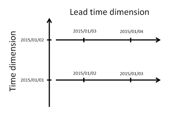
Schematic of how we use the lead-time dimension to store multiple forecasts in a single netCDF file. The lead-time dimension is defined in relation to the time dimension, and means we can store many hindcasts in a single file. The files also handle large ensembles, multiple locations and multiple variables.
A huge benefit of using a standardised, well supported and self-describing binary file format is that it makes sharing data incredibly easy. At first, we found this beneficial within our small research group: even though there are only about 10 of us, we each manage to (strongly!) prefer different scripting languages – R, Matlab, Python. All these scripting languages have strong support for netCDF files so it’s very easy to load and manipulate data. The meta-data stored inside the netCDF files makes reviewing old experiments much easier – we find we don’t have to retrace our steps as much or (gulp!) regenerate hindcasts.
We have since had very good experiences with sharing our netCDF files with collaborators outside our group, and the Bureau of Meteorology has adopted our netCDF specification for operational forecasting. On the downside, binary data formats can be restrictive: netCDF is not readable with simple text editors, and this can occlude data from forecast users or collaborators who don’t have the time or inclination to learn scripting languages or other new software.
Of course, there are many other aspects to the issue of data in ensemble forecasting that we can’t cover in a short blog – we haven’t even touched on algorithm efficiency – and so we’d like to hear your data stories:
- Have you faced similar problems with verifying ensemble forecasts?
- Do you prefer other ways of storing data, like HDF5 or databases?
- Do you have different or better ways of crunching and storing your data?
Tell us in the comments!
[1] Who are we kidding – we were geeks already. Shout out to those who saw the tribute to Missy ‘Misdemeanor’ Elliott in the phrase ‘get your geek on’: there’s a fair chance that you may be even geekier than us. (If not, then go on and treat yourself.)
May 10, 2016 at 15:23
Please give us an ncdump -h of one of your files! Would be illuminating.
May 11, 2016 at 01:14
Hi James – here’s one example (stripped of a bit of metadata for this purpose):
netcdf South_Esk_Ens_1hr_Qadj_Ens_201008 {
dimensions:
time = UNLIMITED ; // (31 currently)
lead_time = 231 ;
station = 7 ;
strLen = 30 ;
ens_member = 1000 ;
variables:
double time(time) ;
time:standard_name = “time” ;
time:long_name = “time” ;
time:time_standard = “UTC” ;
time:axis = “t” ;
time:units = “hours since 2010-08-01 21:00:00.0 +0000” ;
int lead_time(lead_time) ;
lead_time:standard_name = “lead time” ;
lead_time:long_name = “forecast lead time” ;
lead_time:axis = “v” ;
lead_time:units = “hours since time of forecast” ;
int station_id(station) ;
station_id:long_name = “station or node identification code” ;
char station_name(station, strLen) ;
station_name:long_name = “station or node name” ;
int ens_member(ens_member) ;
ens_member:standard_name = “ens_member” ;
ens_member:long_name = “ensemble member” ;
ens_member:units = “member id” ;
ens_member:axis = “u” ;
float q_fcast_ens(time, ens_member, station, lead_time) ;
q_fcast_ens:standard_name = “q_fcast_ens” ;
q_fcast_ens:long_name = “forecast streamflow ensemble” ;
q_fcast_ens:units = “m3/s” ;
q_fcast_ens:_FillValue = -9999.f ;
q_fcast_ens:type = 3. ;
q_fcast_ens:type_description = “averaged over the preceding interval” ;
q_fcast_ens:Location_type = “Point” ;
double lat(station) ;
lat:long_name = “latitude” ;
lat:units = “degrees_north” ;
lat:axis = “y” ;
double lon(station) ;
lon:long_name = “longitude” ;
lon:units = “degrees_east” ;
lon:axis = “x” ;
double area(station) ;
area:long_name = “station area” ;
area:units = “sqm” ;
// global attributes:
:title = “Short-term ensemble stream flow forecast” ;
:institution = “CSIRO Land & Water” ;
:source = “SWIFT v1.0 hydrological model forced with BJP-NWP ensemble rainfall.\n”,
:catchment = “South_Esk” ;
:STF_convention_version = 1. ;
:STF_nc_spec = “https://wiki.csiro.au/display/wirada/NetCDF+for+SWIFT” ;
:comment = “” ;
:history = “2013-09-02 14:44:20 +10.0 – File created” ;
May 10, 2016 at 16:13
On a related topic, in NOAA we recently held a workshop on the statistical post-processing of weather forecasts (pre-processing to hydrologists). While there were many issues related to science, there also were issues related to data handling. If readers are interested in the consensus recommendations for how NOAA evolves to handle this, please see
http://www.esrl.noaa.gov/psd/people/tom.hamill/Post-proc-rec2seniorstaff-Jan2016-v5.pptx
(it may take an hour past when this was posted for this file to show up; it needs to sync across our firewall).
You’ll see that we aim to use portable data structures like netCDF in the future and, ideally, to build a national or international community for sharing algorithms, data, and such.
I hope this is helpful, and if you have thoughts or comments, please feel free to e-mail me.
Thanks,
Tom Hamill
August 4, 2016 at 04:03
Thanks Tom for interesting presentations on statistical post-processing. You mentioned in slide 54 that “I haven’t seen any post-processing methods that attempt to correct for errors in the timing of precipitation”.
It seems our post-processing method based on Bayesian joint probability model is able to correct errors in the timing of precipitation. This results was reported in Fig 9 of http://journals.ametsoc.org/doi/full/10.1175/MWR-D-14-00329.1.
May 11, 2016 at 01:37
Thanks Tom – that is super interesting, not just on the need to handle data consistently and efficiently, but also on articulating the more general need for effective post (pre?) processing of climate/NWP forecasts.
May 26, 2016 at 05:27
Really great stuff, thanks both of you.