The Impact of using Ensemble Generator Produced Precipitation Estimates on the Calibration of a Hydrological Model
Contributed by Christopher J. Skinner
The HEPEX Testbed Ensemble Representation of Rainfall Observation and Analysis Uncertainty was introduced in a previous blog post by Tim Bellerby. It aims to address some of the issues with representing uncertainty in precipitation observations by making use of ensemble simulation approaches and in the last few years I have been developing my research relevant to this Testbed, working with satellite rainfall estimates as one of Tim’s doctoral candidates.
The doctoral research I undertook used an ensemble simulation approach to generate an ensemble of modelled rainfall fields over the sparsely gauge Senegal River Basin – using the TAMSAT satellite rainfall estimation algorithm as the basis. Each of the rainfall fields generated was equiprobable and consistent with the input field, but also unique with the difference between the fields indicative of the uncertainty within the satellite rainfall estimate. A catchment estimate of daily precipitation was produced from each ensemble member and then used individually to drive a version of the Pitman lumped hydrological model of the Bakoye catchment, a still relatively large sub-catchment of the wider basin. The combined outputs are used to produce an ensemble prediction of daily discharge.
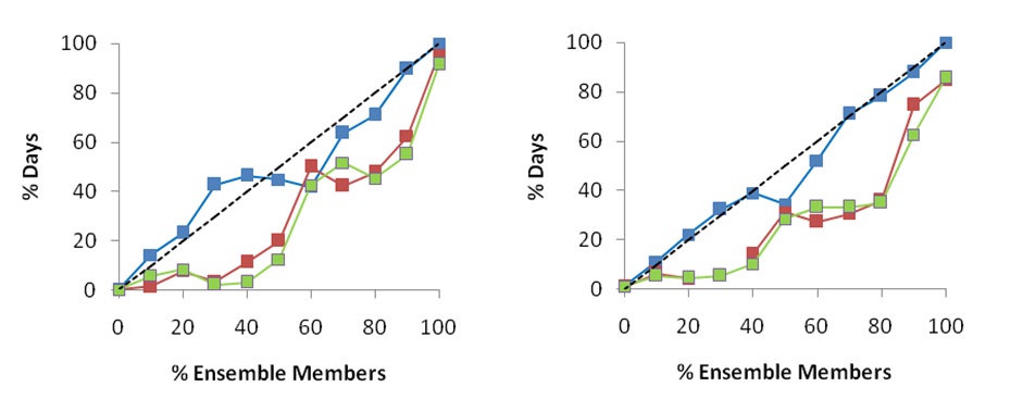
Figure 1 – Discharge Forecast Reliability plots for mean daily discharge volumes in Bakoye catchment, for the calibration period (left) and verification period (right). The red lines show ensemble discharges from the TAMSAT1 calibrated Pitman model, the green from the Pitman model calibrated using the daily mean of the ensembles, EnsMean, and the blue lines shows discharge from the Pitman model calibrated using the EnsAll method.
It is at this point of contact, between the ensemble inputs and a deterministic downstream model, where things get really interesting.
The plots in Figure 1 show the forecast reliability plots for the mean discharge volume, using the same ensemble inputs, but using them to drive the Pitman model with different sets of pre-calibrated parameters. The TAMSAT1 one set of parameters uses a deterministic precipitation estimate based on an adapted version of TAMSAT to produce daily rainfall. EnsMean is the daily mean from the set of ensembles, used as a deterministic estimate – this is statistical similar to TAMSAT1. The final parameter set, EnsAll, uses a novel method that incorporates each ensemble member into the calibration individually but performs the calibration collectively, based on minimising a collective score of error. Each calibration was performed automatically using Shuffled Complex Evolution (SCE-UA).
What was found was that the use of ensemble inputs, produced by an ensemble generator, has implications for model calibration. It is not sufficient to assume that the downstream application can be pre-calibrated by what is considered to be a representative deterministic estimate, as it was seen that even using a mean of the ensembles for the calibration results in a loss of forecast reliability – there was also a general loss in model performance. Although an ensemble based approach is ideally required with regards to the model structure and parameter uncertainty of the downstream model, this needs to be based on the full set of ensemble inputs as individual estimates and not a deterministic estimate.
This is just one aspect of what Tim described as the “enormous unexplored potential in this topic”, and as this field, and the Testbed, takes off and grows it will become increasingly important to understand the influences of using ensemble inputs to drive, and calibrate, downstream environmental models.
If you would like to know more I will be presenting a poster on this on Tuesday, April 29, at EGU 2014 in the session Precipitation: from measurement to modelling and application in catchment hydrology. More results from this research will also be presented in a paper that is currently in the process of submission to the Journal of Hydrology.
April 20, 2014 at 22:14
Great results! Just a little nitty-gritty comment: people will always be curious about the frequencies of different probability classes. Does the 80% probability class contain 3 or 30 cases? A common habit is to show that in a small staple diagram where there is space left (upper left?)
April 22, 2014 at 09:54
Thank you, Anders. Yes, you’re right, and I have these on the figures prepared for the paper (plus a lot more detail).
On another note – last week my poster at EGU was moved to an oral slot on the Monday, 14:30, in Rm 6.