Lessons from calibrating a global flood forecasting system
Contributed by Feyera Hirpa, University of Oxford.
Hydrological models are key tools for predicting flood disasters several days ahead of their occurrence. However, their usability as a decision support tool depends on their skill in reproducing the observed streamflow. The forecast skill is subject to a cascade of uncertainties originating from errors in the models’ structure, parametrization, initial conditions and meteorological forcing.
The Global Flood Awareness System (GloFAS) is an operational flood forecasting system that produces ensemble streamflow forecasts with up to 30-days lead-time and flood exceedance probabilities for major rivers worldwide. It has been running since 2011, becoming fully operational as a 24/7 supported service in April 2018, and is part of the Copernicus Emergency Management Service. For many countries without a local forecasting system, the GloFAS forecasts, which are freely available, may be the only real-time flood forecast information available. This means that improving the forecast skill can potentially have important implications for planning disaster responses.
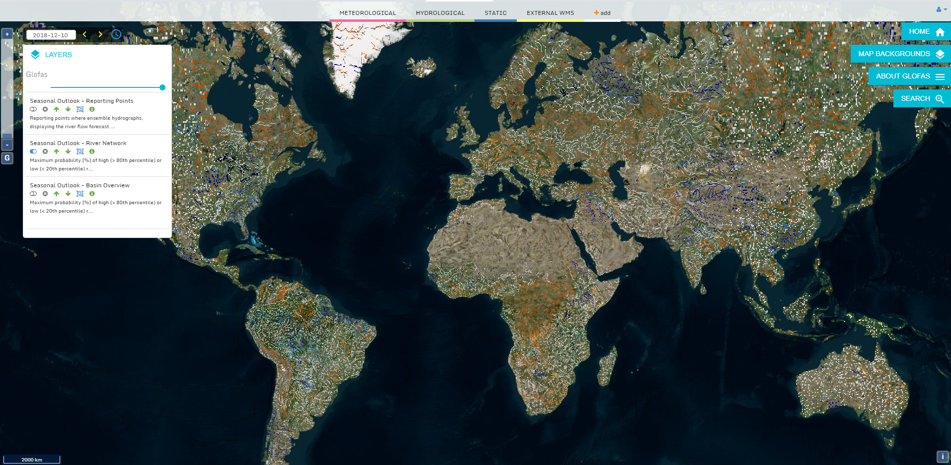
Screenshot of the GloFAS forecast interface at www.globalfloods.eu
More than two years ago, at the Joint Research Centre (JRC) of the European Commission, we took on the task of improving GloFAS flood forecasts by calibrating the underlying hydrological model using daily streamflow data. We started with LISFLOOD, a model that performs runoff routing and groundwater modelling at a daily time step and on a 0.1o resolution river network. In GloFAS, the surface and sub-surface runoff are generated by ECMWF’s land surface scheme HTESSEL. At the time, LISFLOOD used mostly uniform parameter sets for all rivers around the world. We selected the ECMWF reforecast (1995-2015) for model forcing since it is produced by the latest weather model and, therefore, is consistent with the operational weather forecasts.
Here I share my experiences of calibrating the global-scale model, which was a fun task. The idea of improving the skill of an operational flood forecasting system, and thereby contributing to global flood risk reduction, is hugely exciting. The unfolding flood disasters over the last couple of years (e.g, Malawi, Myanmar) certainly served as additional motivations. Learning the hydro-climate of tens of river basins around the world is also cool!
Streamflow data
With the Floods team at the JRC, we started with creating a streamflow observations database. This was the biggest challenge, as it is difficult to access daily (or sub-daily) streamflow data in large parts of the world, and they simply do not exist in some other regions. The Global Runoff Data Centre is the primary source of streamflow data, but the number of stations with daily data is limited and has steadily declined in recent decades. Only a few countries make their streamflow data freely accessible online (e.g., USA and South Africa) and often none of them are in commonly flood-prone regions.
After collecting streamflow data from GRDC, R-ArcticNet database for the Arctic region, and some national databases, we manually checked the data quality, the reported location (if it falls on the model river network) and catchment area (if it is comparable with the modelled upstream area) for each of the gauging stations. The data, which should overlap with the forcing period (1995-2015), was split into two parts for calibration (the most recent period) and validation. We set the data length for calibration to a minimum of 4 years and a maximum of 8 years (to save computational time). In total, daily streamflow data from 1287 stations were used.
Calibration methods
Calibration of a global-scale distributed model needs an efficient and effective algorithm that can converge within a reasonable time. A Non-dominated Sorting Genetic Algorithm fits the bill since it rapidly converges to a best performing parameter sets. It is a population-based optimization algorithm that modifies the population through evolution over a range of generations and, ultimately, identifies the best performing individual (a set of model parameters). The algorithm was implemented using Python programming language as a Distributed Evolutionary Algorithm in Python (DEAP), which enables parallel simulations on multiple cores. We selected the Kling-Gupta efficiency (KGE; Eq. 9 in this paper) as the objective function since it combines bias, correlation and variability in one function. The selected configuration takes, on average, about 6 hours to complete for each of the 1287 calibration stations on a 12-core machine. To accelerate the calibration process, we divided the task on multiple machines.
When multiple stations exist in a given basin, we calibrated the interstation regions in order from upstream to downstream (in ascending catchment area), with outflows from the calibrated upstream sub-basin used as inflow to the interstation region. This means that each of the interstation regions and the upstream sub-basin all having a unique set of parameters after calibration. Figure 1 shows a streamflow time series during the calibration and validation periods for a selected station.
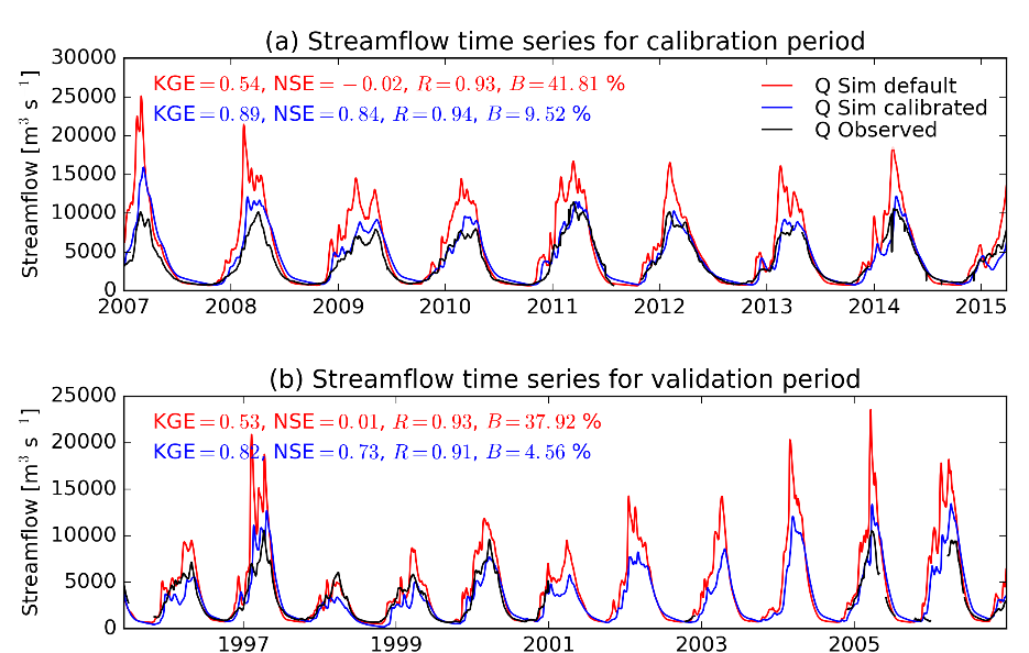
Figure 1. Streamflow time series for a selected station (Xingu river at Boa Sorte in Brazil, Upstream area 206,800 km2)
Lessons learned
The following are the main lessons learned from calibrating and evaluating GloFAS:
- Calibrating LISFLOOD parameters related to the flow timing, variability and groundwater loss has overall improved the streamflow simulation. However, the skill gain varies regionally, with South America and Africa having the largest skill gain and North America the smallest (Figure 2).
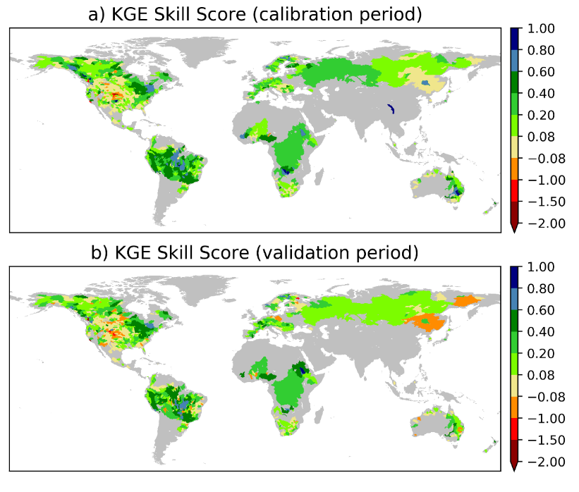
Figure 2. The Kling-Gupta Efficiency Skill Score.
- The skill gain varies with the bias in the baseline streamflow (produced using default LISFLOOD parameters, i.e., without calibration, Figure 3). The largest streamflow improvements occurred in areas with positive bias in the baseline streamflow, while the lowest skill score was obtained in basins with a negative bias. This is linked to the GloFAS configuration in which LISFLOOD is used for runoff routing and groundwater modelling, which limits the ability of the model to correct the negative bias.

Figure 3. The skill score variation with bias in the baseline simulation.
- Further improvement of GloFAS forecast skill requires calibration of additional parameters responsible for runoff generation, and reducing bias in the meteorological forecasts. Moreover, future calibration work may take advantage of the ever-improving remotely sensed data, the rapidly increasing computation capacity, and potential advances in calibration algorithms.
- The final lesson (which is very important but not included in scientific publications) is that it is always good to be prepared for the “unpleasant surprises”, especially when running ~1300 simulations each requiring 6 hours to complete. A small bug in the calibration or model code may require starting a 325 PC days long simulation all over again!
I am grateful to the JRC team, led by Dr. Peter Salamon, for the opportunity to learn from this rewarding experience. And I would like to congratulate all who have contributed to the latest GloFAS upgrade. A detailed description of the calibration work can be found here. Finally, thanks go to the centres that maintain and share streamflow data, without which this work would not have been done.
0 comments