A course on probability
by Anders Persson
The lecture series was first given as a 5-day course in Bologna, Italy in February 2015. Here are the presentations in PDF with a short introduction explaining why this particular lecture is relevant. You can download the lectures individually, or all lectures here: All Lectures. The course in Bologna was also filmed, and the videos are available here.
Day 1: Classical probabilities
- Lecture_1 Why probabilities? The reasons why probabilities or uncertainty information is still crucial in spite of the gradual increasing in the quality of deterministic forecasts
- Lecture_2 The power of randomness: The reason why statistics in general and probabilities in particular were late on the scientific stage is because Man has believed that there is no randomness because everything is decided by supernatural forces
- Lecture_3 Adding or combining probabilities: This lecture is motivated by encounters over the years with meteorological colleagues who have underestimated the complexity of combing probabilities.
- Lecture_4 Markov chains: This is one of my “babies” which not only tells us more about combing dependent probabilities but also constitute a miniature model of forecasting in general
Day 2: Frequentist probabilities
- Lecture_5 The problem with the mean: The most mathematically trivial of all statistical equations, The Mean, offers many opportunities to draw the wrong conclusions. This is also true for the slightly more complicated root mean square error.
- Lecture_6 Verification of probability forecasts: Frequentist statistics deals with analyses of historical data, in our science preferably observational records and verification of forecasts.
- Lecture_7 Forecast system validation: While “verification” in our science means evaluating the forecast accuracy (skill, hit rate etc), “validation” concerns the realism of the statistical properties (the mean error, the variance etc).
- Lecture_8 Statistical interpretation and calibration: From verification and validation there is only a small step to make use of this statistical information to modify the forecasts by removing systematic and damping non-systematic errors.
Day 3: Subjective or Bayesian probabilities
- Lecture_9 Bayesianism: The controversial “Bayesian statistics” is given a light hearted presentation including Siméon de Laplace’s “Rule of Succession” (Will the sun rise tomorrow?) and James Bond’s devise “Never say never”.
- Lecture_10 Bayesianism according to Bayes: Thomas Bayes (1701-61) was an English reverend who left his ideas in his last will. His idea of rolling balls over a billiard table is in my view the best explanation of Bayesianism.
- Lecture_11 Conclusions from small samples: From a practical point of view, Bayesian statistics provides some advantages when drawing probabilistic conclusions from small samples or limited experiences.
- Lecture_12 Adaptive Kalman filtering: The statistical interpretation mostly use a frequentist approach (as in MOS) but a Bayesian approach has it advantages in a changing environment with repeated model updates.
Day 4: Decision making using probabilities
- Lecture_13 Decision making from probabilities: The usefulness of probability forecasts is shown by a rather extreme example where the forecasters, when they are uncertain, add value by not issuing any forecasts at all!
- Lecture_14 Some complications in the decision process: It is shown that the “best” forecasts in a statistical sense are not necessarily the most useful and that the “school book” cost-loss model is just an elementary, first approximation.
- Lecture_15 Communicating probabilities: Seven ways to communicate probabilities using concepts as “base rate”, “framing” and other “tricks” to enable the receivers of the information make the best decision.
- Lecture_16 Probability products: Finally an overview of the products from the ECMWF ensemble system and how to interpret them. Combinations of probabilities with ensemble mean maps are recommended.
Day 5: The psychology of probabilities
- Lecture_17 Common pitfalls in probability forecasting: Over confidence, neglect to consider the Base Rate, the Conformation Bias, the Representativity and Availability Effects and other psychological pitfalls might influence the assessments of probabilities.
- Lecture_18 Conditional probabilities: Although we all realise that the probability of an hydrologist having a driver’s licence is much more likely than that someone with a driver’s licence is a hydrologist, conditional probability is yet a source of frequent misinterpretations, sometimes even with fatal consequences.
- Lecture_19 The regression to the mean effect: This is an even more lethal statistical artefacts causing fatal misjudgement among both forecasters and scientists. It even affects our daily life, for example the conclusion that if people improve after having been criticised, it is because of the criticism!
- Lecture_20 Summary of the course:
Lab sessions
We also had plans for simple “lab sessions” using the so called “Trento Dice”:
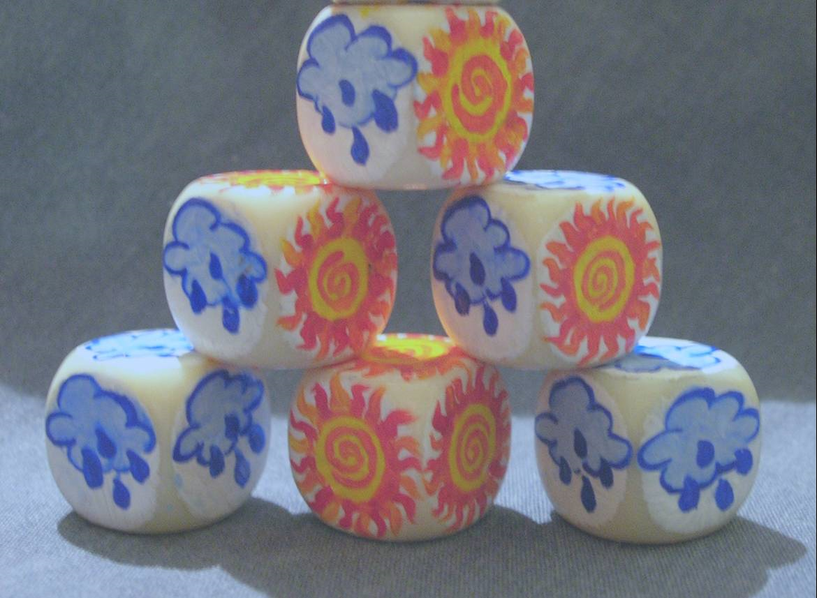
The six dice constructed for the Trento meteorological winter course in 2005. Each dice has 1, 2, 3, 4, 5 or 6 rain clouds (alternative blazing sun shine). A copy was later made using Finnish wood and decorated by an English artist in Norrköping, Sweden. The set was lent to the WMO and ECMWF training courses where it has been used with great success thereafter.
On Day 1 we compared the relative frequency of “sun shine” and “rain cloud” outcomes when just one dice, for example the two “rain cloud” dice, was cast. To simulate auto-correlation an additional dice was used with four “rain cloud”. When the latter came up with “sun shine” the other was used. When it showed “rain cloud” the thrower went back to the first dice.
On Day 2 we had plans to throw one dice repeatedly and see how long it took for the relative frequency to stabilize around the “correct” value.
On Day 3 a dice was randomly selected and cast. For every throw Bayes Rule was used to estimate probabilities for the most likely dice to have been chosen.
On Day 4 we intended to play the “2005 Trento Game” simulating the cost-loss model, the game that has been used on numerous WMO and ECMWF courses the last ten years.
Finally on Day 5 a dice was chosen at random and hidden. The question was asked about the probability that it would, thrown twice, show the same symbols? The participants, confusing the question with the problem of getting two rain symbols or two sun shine symbols, thought that the question was impossible to answer since the dice was hidden. But they were then easily convinced that, against what psychologically could be expected the probability is exactly 2/3.
See also the blog post ‘How to bring out the “intuitive statistician” in every forecaster’ here.
March 23, 2015 at 23:51
The pdf lectures are a jewel however many of them have some problems when opening and reading them with any Adobe Reader Aplication. It is possible to repair them. Thanks a lot for share these valuos material.
March 24, 2015 at 15:40
Dear David,
Thanks for pointing it out. We have fixed the damage files that we found. Please let us know if there are any more problems with them. You can now also download all files in one zipped folder.
Cheers,
Fredrik